NMF 分解的自定义算子¶

NMF 将输入矩阵分解为两个秩为 k 的矩阵 W, H，使得 $WH \sim M`$ 。 $M=(m_{ij})$ 可以是一个二元矩阵，其中 i 代表用户，j 代表他购买的产品。预测函数取决于用户是需要为现有用户还是新用户进行推荐。本示例处理第一种情况。

第二种情况更复杂，因为它理论上需要通过梯度下降来估计一个新的矩阵 W。

构建一个简单的模型¶

import os
import skl2onnx
import onnxruntime
import sklearn
from sklearn.decomposition import NMF
import numpy as np
import matplotlib.pyplot as plt
from onnx.tools.net_drawer import GetPydotGraph, GetOpNodeProducer
import onnx
from skl2onnx.algebra.onnx_ops import OnnxArrayFeatureExtractor, OnnxMul, OnnxReduceSum
from skl2onnx.common.data_types import FloatTensorType
from onnxruntime import InferenceSession


mat = np.array(
    [[1, 0, 0, 0], [1, 0, 0, 0], [1, 0, 0, 0], [1, 0, 0, 0], [1, 0, 0, 0]],
    dtype=np.float64,
)
mat[: mat.shape[1], :] += np.identity(mat.shape[1])

mod = NMF(n_components=2)
W = mod.fit_transform(mat)
H = mod.components_
pred = mod.inverse_transform(W)

print("original predictions")
exp = []
for i in range(mat.shape[0]):
    for j in range(mat.shape[1]):
        exp.append((i, j, pred[i, j]))

print(exp)

original predictions
[(0, 0, np.float64(1.8940619439633473)), (0, 1, np.float64(0.3072432913109815)), (0, 2, np.float64(0.1091000464503179)), (0, 3, np.float64(0.3072432913109815)), (1, 0, np.float64(1.1066037222104155)), (1, 1, np.float64(0.19083096278248987)), (1, 2, np.float64(0.0)), (1, 3, np.float64(0.19083096278248987)), (2, 0, np.float64(1.014668907902116)), (2, 1, np.float64(0.0)), (2, 2, np.float64(0.9848932612757917)), (2, 3, np.float64(0.0)), (3, 0, np.float64(1.1066037222104155)), (3, 1, np.float64(0.19083096278248987)), (3, 2, np.float64(0.0)), (3, 3, np.float64(0.19083096278248987)), (4, 0, np.float64(0.9470309719816736)), (4, 1, np.float64(0.15362164565549075)), (4, 2, np.float64(0.05455002322515895)), (4, 3, np.float64(0.15362164565549075))]

让我们改写预测函数，使其更接近我们需要转换为 ONNX 的函数。

def predict(W, H, row_index, col_index):
    return np.dot(W[row_index, :], H[:, col_index])


got = []
for i in range(mat.shape[0]):
    for j in range(mat.shape[1]):
        got.append((i, j, predict(W, H, i, j)))

print(got)

[(0, 0, np.float64(1.8940619439633473)), (0, 1, np.float64(0.3072432913109815)), (0, 2, np.float64(0.1091000464503179)), (0, 3, np.float64(0.3072432913109815)), (1, 0, np.float64(1.1066037222104155)), (1, 1, np.float64(0.19083096278248987)), (1, 2, np.float64(0.0)), (1, 3, np.float64(0.19083096278248987)), (2, 0, np.float64(1.014668907902116)), (2, 1, np.float64(0.0)), (2, 2, np.float64(0.9848932612757917)), (2, 3, np.float64(0.0)), (3, 0, np.float64(1.1066037222104155)), (3, 1, np.float64(0.19083096278248987)), (3, 2, np.float64(0.0)), (3, 3, np.float64(0.19083096278248987)), (4, 0, np.float64(0.9470309719816736)), (4, 1, np.float64(0.15362164565549075)), (4, 2, np.float64(0.05455002322515895)), (4, 3, np.float64(0.15362164565549075))]

转换为 ONNX¶

目前没有实现 NMF 的转换器，因为我们计划转换的函数既不是 transformer 也不是 predictor。下面的转换器不需要注册，它只是创建一个等同于上面实现的 predict 函数的 ONNX 图。

def nmf_to_onnx(W, H, op_version=12):
    """
    The function converts a NMF described by matrices
    *W*, *H* (*WH* approximate training data *M*).
    into a function which takes two indices *(i, j)*
    and returns the predictions for it. It assumes
    these indices applies on the training data.
    """
    col = OnnxArrayFeatureExtractor(H, "col")
    row = OnnxArrayFeatureExtractor(W.T, "row")
    dot = OnnxMul(col, row, op_version=op_version)
    res = OnnxReduceSum(dot, output_names="rec", op_version=op_version)
    indices_type = np.array([0], dtype=np.int64)
    onx = res.to_onnx(
        inputs={"col": indices_type, "row": indices_type},
        outputs=[("rec", FloatTensorType((None, 1)))],
        target_opset=op_version,
    )
    return onx


model_onnx = nmf_to_onnx(W.astype(np.float32), H.astype(np.float32))
print(model_onnx)

ir_version: 7
producer_name: "skl2onnx"
producer_version: "1.19.1"
domain: "ai.onnx"
model_version: 0
graph {
  node {
    input: "Ar_ArrayFeatureExtractorcst"
    input: "col"
    output: "Ar_Z0"
    name: "Ar_ArrayFeatureExtractor"
    op_type: "ArrayFeatureExtractor"
    domain: "ai.onnx.ml"
  }
  node {
    input: "Ar_ArrayFeatureExtractorcst1"
    input: "row"
    output: "Ar_Z02"
    name: "Ar_ArrayFeatureExtractor1"
    op_type: "ArrayFeatureExtractor"
    domain: "ai.onnx.ml"
  }
  node {
    input: "Ar_Z0"
    input: "Ar_Z02"
    output: "Mu_C0"
    name: "Mu_Mul"
    op_type: "Mul"
    domain: ""
  }
  node {
    input: "Mu_C0"
    output: "rec"
    name: "Re_ReduceSum"
    op_type: "ReduceSum"
    domain: ""
  }
  name: "OnnxReduceSum"
  initializer {
    dims: 2
    dims: 4
    data_type: 1
    float_data: 1.97398615
    float_data: 0.340408832
    float_data: 0
    float_data: 0.340408832
    float_data: 0.89287746
    float_data: 0
    float_data: 0.866675794
    float_data: 0
    name: "Ar_ArrayFeatureExtractorcst"
  }
  initializer {
    dims: 2
    dims: 5
    data_type: 1
    float_data: 0.90257144
    float_data: 0.560593426
    float_data: 0
    float_data: 0.560593426
    float_data: 0.45128572
    float_data: 0.125883341
    float_data: 0
    float_data: 1.13640332
    float_data: 0
    float_data: 0.0629416704
    name: "Ar_ArrayFeatureExtractorcst1"
  }
  input {
    name: "col"
    type {
      tensor_type {
        elem_type: 7
        shape {
          dim {
          }
        }
      }
    }
  }
  input {
    name: "row"
    type {
      tensor_type {
        elem_type: 7
        shape {
          dim {
          }
        }
      }
    }
  }
  output {
    name: "rec"
    type {
      tensor_type {
        elem_type: 1
        shape {
          dim {
          }
          dim {
            dim_value: 1
          }
        }
      }
    }
  }
}
opset_import {
  domain: ""
  version: 12
}
opset_import {
  domain: "ai.onnx.ml"
  version: 1
}

让我们用它来计算预测。

sess = InferenceSession(
    model_onnx.SerializeToString(), providers=["CPUExecutionProvider"]
)


def predict_onnx(sess, row_indices, col_indices):
    res = sess.run(None, {"col": col_indices, "row": row_indices})
    return res


onnx_preds = []
for i in range(mat.shape[0]):
    for j in range(mat.shape[1]):
        row_indices = np.array([i], dtype=np.int64)
        col_indices = np.array([j], dtype=np.int64)
        pred = predict_onnx(sess, row_indices, col_indices)[0]
        onnx_preds.append((i, j, pred[0, 0]))

print(onnx_preds)

[(0, 0, np.float32(1.8940619)), (0, 1, np.float32(0.3072433)), (0, 2, np.float32(0.109100044)), (0, 3, np.float32(0.3072433)), (1, 0, np.float32(1.1066036)), (1, 1, np.float32(0.19083095)), (1, 2, np.float32(0.0)), (1, 3, np.float32(0.19083095)), (2, 0, np.float32(1.014669)), (2, 1, np.float32(0.0)), (2, 2, np.float32(0.98489326)), (2, 3, np.float32(0.0)), (3, 0, np.float32(1.1066036)), (3, 1, np.float32(0.19083095)), (3, 2, np.float32(0.0)), (3, 3, np.float32(0.19083095)), (4, 0, np.float32(0.94703096)), (4, 1, np.float32(0.15362164)), (4, 2, np.float32(0.054550022)), (4, 3, np.float32(0.15362164))]

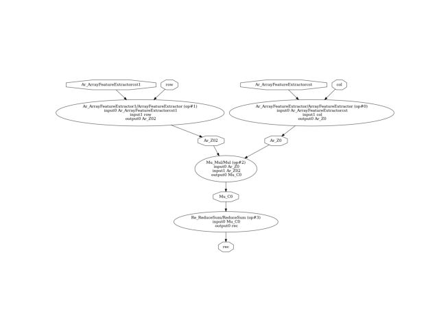
ONNX 图如下所示。

pydot_graph = GetPydotGraph(
    model_onnx.graph,
    name=model_onnx.graph.name,
    rankdir="TB",
    node_producer=GetOpNodeProducer("docstring"),
)
pydot_graph.write_dot("graph_nmf.dot")
os.system("dot -O -Tpng graph_nmf.dot")
image = plt.imread("graph_nmf.dot.png")
plt.imshow(image)
plt.axis("off")

(np.float64(-0.5), np.float64(1654.5), np.float64(846.5), np.float64(-0.5))

此示例使用的版本

print("numpy:", np.__version__)
print("scikit-learn:", sklearn.__version__)
print("onnx: ", onnx.__version__)
print("onnxruntime: ", onnxruntime.__version__)
print("skl2onnx: ", skl2onnx.__version__)

numpy: 2.3.1
scikit-learn: 1.6.1
onnx:  1.19.0
onnxruntime:  1.23.0
skl2onnx:  1.19.1

脚本总运行时间： (0 分钟 0.454 秒)

Sphinx-Gallery 生成的图库