比较 CDist 与 scipy

以下示例重点介绍一个特定的操作符 CDist，并比较它在 onnxruntime 和 scipy 之间的执行时间。

包含 CDist 的 ONNX 图

cdist 函数计算成对距离。

from pprint import pprint
from timeit import Timer
import numpy as np
from scipy.spatial.distance import cdist
from tqdm import tqdm
from pandas import DataFrame
import onnx
import onnxruntime as rt
from onnxruntime import InferenceSession
import skl2onnx
from skl2onnx.algebra.custom_ops import OnnxCDist
from skl2onnx.common.data_types import FloatTensorType

X = np.ones((2, 4), dtype=np.float32)
Y = np.ones((3, 4), dtype=np.float32)
Y *= 2
print(cdist(X, Y, metric="euclidean"))

[[2. 2. 2.]
 [2. 2. 2.]]

ONNX

op = OnnxCDist("X", "Y", op_version=12, output_names=["Z"], metric="euclidean")
onx = op.to_onnx({"X": X, "Y": Y}, outputs=[("Z", FloatTensorType())])
print(onx)

ir_version: 10
producer_name: "skl2onnx"
producer_version: "1.18.0"
domain: "ai.onnx"
model_version: 0
graph {
  node {
    input: "X"
    input: "Y"
    output: "Z"
    name: "CD_CDist"
    op_type: "CDist"
    attribute {
      name: "metric"
      s: "euclidean"
      type: STRING
    }
    domain: "com.microsoft"
  }
  name: "OnnxCDist"
  input {
    name: "X"
    type {
      tensor_type {
        elem_type: 1
        shape {
          dim {
          }
          dim {
            dim_value: 4
          }
        }
      }
    }
  }
  input {
    name: "Y"
    type {
      tensor_type {
        elem_type: 1
        shape {
          dim {
          }
          dim {
            dim_value: 4
          }
        }
      }
    }
  }
  output {
    name: "Z"
    type {
      tensor_type {
        elem_type: 1
      }
    }
  }
}
opset_import {
  domain: "com.microsoft"
  version: 1
}

CDist 与 onnxruntime

我们使用 onnxruntime 计算 CDist 操作符的输出。

sess = InferenceSession(onx.SerializeToString(), providers=["CPUExecutionProvider"])
res = sess.run(None, {"X": X, "Y": Y})
print(res)

[array([[1.9999999, 1.9999999, 1.9999999],
       [1.9999999, 2.       , 2.       ]], dtype=float32)]

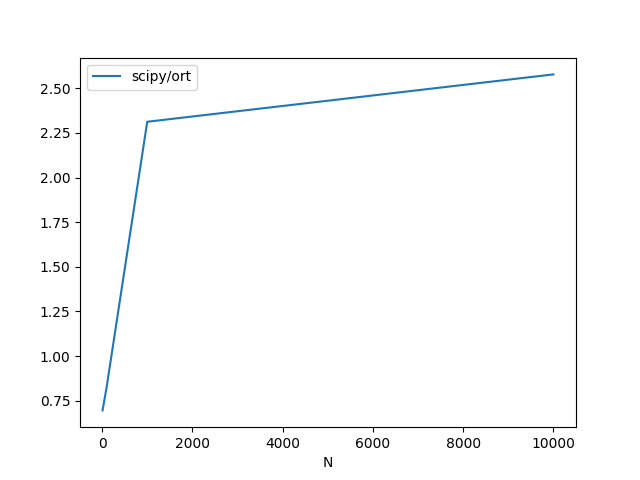
基准测试

让我们比较 onnxruntime 和 scipy。

def measure_time(name, stmt, context, repeat=100, number=20):
    tim = Timer(stmt, globals=context)
    res = np.array(tim.repeat(repeat=repeat, number=number))
    res /= number
    mean = np.mean(res)
    dev = np.mean(res**2)
    dev = (dev - mean**2) ** 0.5
    return dict(
        average=mean,
        deviation=dev,
        min_exec=np.min(res),
        max_exec=np.max(res),
        repeat=repeat,
        number=number,
        nrows=context["X"].shape[0],
        ncols=context["Y"].shape[1],
        name=name,
    )

scipy

time_scipy = measure_time(
    "scipy", "cdist(X, Y)", context={"cdist": cdist, "X": X, "Y": Y}
)
pprint(time_scipy)

{'average': np.float64(8.157823500368977e-06),
 'deviation': np.float64(8.986884053687116e-06),
 'max_exec': np.float64(5.3478249901672827e-05),
 'min_exec': np.float64(2.6912999601336197e-06),
 'name': 'scipy',
 'ncols': 4,
 'nrows': 2,
 'number': 20,
 'repeat': 100}

onnxruntime

time_ort = measure_time(
    "ort", "sess.run(None, {'X': X, 'Y': Y})", context={"sess": sess, "X": X, "Y": Y}
)
pprint(time_ort)

{'average': np.float64(3.3001529995090104e-05),
 'deviation': np.float64(3.1202860470685634e-05),
 'max_exec': np.float64(0.00018513064987928373),
 'min_exec': np.float64(6.747400038875639e-06),
 'name': 'ort',
 'ncols': 4,
 'nrows': 2,
 'number': 20,
 'repeat': 100}

更长的基准测试

metrics = []
for dim in tqdm([10, 100, 1000, 10000]):
    # We cannot change the number of column otherwise
    # we need to create a new graph.
    X = np.random.randn(dim, 4).astype(np.float32)
    Y = np.random.randn(10, 4).astype(np.float32)

    time_scipy = measure_time(
        "scipy", "cdist(X, Y)", context={"cdist": cdist, "X": X, "Y": Y}
    )
    time_ort = measure_time(
        "ort",
        "sess.run(None, {'X': X, 'Y': Y})",
        context={"sess": sess, "X": X, "Y": Y},
    )
    metric = dict(N=dim, scipy=time_scipy["average"], ort=time_ort["average"])
    metrics.append(metric)

df = DataFrame(metrics)
df["scipy/ort"] = df["scipy"] / df["ort"]
print(df)

df.plot(x="N", y=["scipy/ort"])

  0%|          | 0/4 [00:00<?, ?it/s]
 75%|███████▌  | 3/4 [00:00<00:00, 12.27it/s]
100%|██████████| 4/4 [00:01<00:00,  2.39it/s]
       N     scipy       ort  scipy/ort
0     10  0.000010  0.000011   0.970933
1    100  0.000009  0.000009   1.026960
2   1000  0.000060  0.000021   2.846234
3  10000  0.000576  0.000137   4.211802

本例使用的版本

print("numpy:", np.__version__)
print("onnx: ", onnx.__version__)
print("onnxruntime: ", rt.__version__)
print("skl2onnx: ", skl2onnx.__version__)

numpy: 2.2.0
onnx:  1.18.0
onnxruntime:  1.21.0+cu126
skl2onnx:  1.18.0